Companies in natural-resource-based industries depend heavily on commodity price forecasts to make major strategic decisions, such as whether to construct a new mine or expand production at an existing mine. The price they can get for the commodities they produce will have a huge impact on their revenues and profits, so it powerfully influences their choices.
Price also factors heavily into companies’ liquidity planning. For instance, owing to required fair-value assessments, companies can easily run into debt covenant violations if prices plummet unexpectedly and they have to initiate an equity write-down. Finally, investors and trading companies rely on price forecasts to determine where to place their biggest bets, whether they be on commodity-based financial products or on mining assets.
Despite this dependence on commodity price forecasts, it’s extremely difficult—if not impossible—to predict what a ton of iron ore, an ounce of gold, or a ton of copper will sell for tomorrow, next month, or next year. This has always been true, but increased volatility in commodity markets has made forecasting more challenging than ever. Market observers tend to assume that past patterns of a commodity’s price will continue into the future, and they deliver a single outlook extrapolated from past price behavior.
To overcome the inherent difficulties in forecasting commodity prices , natural-resource-based companies and investors need to develop a more nuanced view of the markets they’re playing in. Such a view can help them form their own opinion of where prices will go and what it will mean for the strategic decisions they face. We recommend a four-step process for developing a range of scenarios based on in-depth supply-and-demand modeling.
Step 1: Understand Your Market’s Most Powerful Drivers
In every commodity market, price is powerfully influenced by supply-and-demand dynamics, which, in turn, are subject to a set of drivers. Supply, for instance, is driven by the production profiles of existing mines, the ramp-up of new mines, recycling activity, and mining production costs. Demand drivers include general macroeconomic development (such as China’s rise during the last decade) and consumer behavior (such as Chinese consumers’ increasing sensitivity to price in the purchase of gold jewelry). The value of a commodity’s specific characteristics in manufacturing processes also affects demand. So do the prices of close substitutes: when they decrease, demand for the original commodity wanes.
Complicating things further, supply and demand drivers are not only interdependent but also subject to price. That is, price affects them as much as they influence price. What’s more, these drivers are always changing, sometimes in response to major unexpected events. Examples include export bans imposed by a producing country’s regime or a disruptive technology that makes a particular commodity obsolete in a key application.
Price sensitivity to changes in supply and demand drivers varies substantially across commodities and across the users of a given commodity. To investigate this, we conducted a sensitivity analysis for copper, gold, and iron ore using
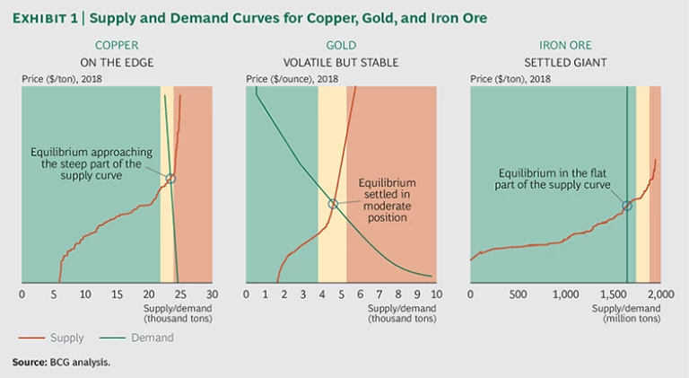
What explains such differences in price sensitivity to the same underlying drivers? The disparities stem from variations in a metal’s supply and demand curves, along with the location of the equilibrium point (the intersection of supply and demand) on those curves. (See Exhibit 1.) With copper, for example, our analysis shows that, by 2018, the equilibrium point will “settle” in a steep section of the supply curve. Consequently, we anticipate that even a small change in supply or demand will have a disproportionately large impact on the price of copper. When supply-and-demand equilibrium settles at a moderately pitched point on the supply curve (as our analysis indicates for gold in 2018), price reacts less extremely to changes in supply or demand drivers. And when the equilibrium point settles at a fairly flat part of the supply curve (as we anticipate for iron ore in 2018), even major changes in supply or demand will have little impact on the commodity’s price.
All this has important implications for industry players. Given that supply-and-demand dynamics vary so widely across different commodities—and that such differences strongly influence commodity prices—companies and investors need to identify the supply and demand drivers that most affect their commodity of interest. To be sure, certain drivers (such as GDP development and factor cost inflation) influence almost all commodities (though to differing degrees). But each commodity has its own specific and often unique drivers. Take gold. Two of the most powerful drivers in this market are the expected level of investor demand resulting from economic uncertainty and the degree of price sensitivity in Asian markets. While strongly influencing the price of gold, those two drivers have limited (if any) impact on copper and iron ore prices. Meanwhile, specific drivers for the copper and iron ore markets are more tied to substitution trends and the intensity of infrastructure development.
Step 2: Develop Base, Upside, and Downside Cases
By developing a set of scenarios representing potential changes in supply and demand drivers for their commodity of interest, industry players can make more informed judgments about the likelihood of major deviations from base-case price forecasts. The scenarios cover a range of possible developments and reflect the key drivers affecting specific markets.
Companies and investors start from a base case, which usually takes the consensus view of how the commodity’s supply-and-demand environment may evolve. They then develop two “bookend” scenarios: an upside and a downside case showing an environment conducive to a favorable and an unfavorable price, respectively. Depending on the purpose of the analysis, the time horizon can be short (two or three years to define operational priorities for an asset) or long (ten years or more to inform a project development decision).
To be most useful, the bookend scenarios should represent extreme conditions, not just slight modifications from the base case. Moreover, they need to be based on feasible assumptions about how supply and demand drivers might actually change, rather than on formulaic adjustments to the base case (such as 10 percent above and below the base-case price). Finally, by giving the scenarios names that paint an easy-to-envision picture of the future, industry players can more easily discuss and refer to these scenarios during strategy sessions.
To help illustrate how the three scenarios come into play, let’s focus on the iron ore market, drawing on scenarios developed from CMI modeling. According to our analysis, the base case for this market—which we call “soft landing in China”—will be characterized by a modest slowing of growth in China’s GDP (5.3 percent in 2020 and 3.8 percent in 2025), moderate project volume growth, and slight increases in production costs (3.5 percent annually). The upside case—“China’s second rise”—shows strong reacceleration of China’s GDP growth (9.5 percent by 2025) driven by renewed emphasis on government-led infrastructure programs. This scenario also anticipates more mine expansions and greenfield projects initiated to meet strong demand for iron ore. In the downside case—“the Chinese bubble bursts”—we envision a significant decline in China’s GDP (3.5 percent in 2020 and 2.9 percent in 2025) and a larger share of GDP being driven by consumption. All of this would create a compounded negative effect on iron ore demand.
Step 3: Simulate Price Behavior for Each Case
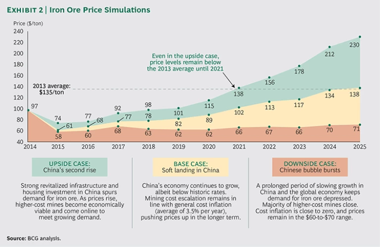
Simulating price behavior for the base, upside, and downside cases requires the application of a recursive market model that takes into account how supply- and demand-side players would respond to changes in market prices. (See Exhibit 2.) Returning to our iron ore example, there is almost no price-related short-term elasticity in demand for this commodity. Demand is driven primarily by demand for steel, which, in turn, is powered by economic growth and construction. However, expected price levels certainly affect production decisions.
To reflect this decision-making process on the supply side, we analyzed the production and production cost profiles of more than 2,000 mines over the past 20 years. We found that most mines keep operating for a certain period even if they cannot cover their
As shown in Exhibit 2, the bookend scenarios comprise a wide range of price levels, especially in the medium and longer term. Given the inelasticity of demand in the iron ore market, this price differential is a cause (as well as a consequence) of the decision by individual companies to cease or continue production. For example, in the downside case, many junior mines would be squeezed out of the market. While this effect was already apparent in 2014 and the first half of 2015, the economic realities of the downside case would cause an additional 22 percent of junior mines (over our base case) to exit production in the medium term. Mines in Australia would take the hardest overall hit (about a 50 percent cut). As a result, the already rather consolidated iron ore market would be even more strongly dominated by volumes from the top five companies (Vale, BHP Billiton, Rio Tinto, Fortescue Metals Group, and Anglo American). These giants would account for roughly 80 percent of global seaborne and Chinese domestic supply by 2018 (versus 69 percent in our base case). On the other hand, the upside case shows fragmented volumes from junior mines rising again. This could lead to a decline in the top five’s market share, which could drop below 60 percent by 2018.
Given the peculiarities of the iron ore market, it’s worth taking a moment to elaborate on Chinese producers’ behavior, since domestic production determines the seaborne supply volumes required to meet demand. In our analysis, we differentiate between three general types of mines in China: state-owned assets, privately owned mines close to the coast, and privately owned inland mines. Each type responds differently to volatility in iron ore prices.
For instance, state-owned assets tend to keep operating almost irrespective of cash losses, owing to the Chinese government’s social priorities. These mines would therefore be positioned on the left side of the supply curve, despite their comparably high average production costs. Privately owned producers, on the other hand, act more in line with commercial principles: they cease operation once the AISC-to-price hurdle is breached. This principle holds true for all private mines. But the farther inland a domestic Chinese asset is located, the more it is shielded from seaborne price levels. The reason? The required domestic transport costs from the closest harbor to the receiving steel mill are very high. (Transport costs from the coast to mills located in China’s Xinjiang region can reach $90 per ton.) We account for this in our CMI model by making a distinction between coastal and inland mines. To illustrate, our downside case assumes that almost all of the 140 million tons of coastal capacity will be out of production by 2018 because of price-related closures. Meanwhile, the “shielded” inland volumes will drop by only about 30 percent.
To see what this part of the process might look like in action, let’s suppose that an iron ore mining company or private-equity company is considering purchasing an operating iron ore mine. The potential buyer has already received information regarding some aspects of the deal. For example, it understands that the mine has an annual capacity of 5 million tons and is expected to operate at an AISC of $65 per ton in 2016—the first year under the new owner. The estimated end of the mine’s life is 2025, with production starting to ramp down in 2023. The seller has informed the potential buyer that the process is competitive and has indicated that it will only consider offers above $500 million. The potential buyer requires at least a 12 percent rate of return.
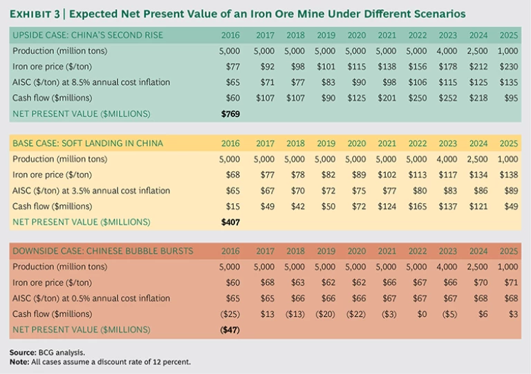
Using this information as well as the price forecasts developed in step 3, our potential buyer can calculate the net present value (NPV) under the different scenarios. (See Exhibit 3.) An NPV above $500 million implies that the mine will meet the buyer’s investment criteria. An NPV below $500 million suggests the opposite.
The outcome varies significantly across the three scenarios. While the NPV is $769 million in the buyer’s upside case, it is only $407 million in the base case and even turns negative at –$47 million in the downside case. Hence, the mine would meet the buyer’s required rate of return only if reality is an improvement over the base case depicted in the “soft landing in China” scenario and is more like the “China’s second rise” scenario. For this potential buyer, the investment decision is very difficult, given that NPV differs so greatly across the scenarios.
Of course, we don’t know the perspective on the Chinese economy and the risk appetite of the mining or private-equity company considering this purchase. However, we can provide some additional relevant information, such as how the world would need to look in order to justify a minimum bid price of $500 million. For the sake of simplicity, let’s use China’s GDP as the key variable. By leveraging BCG’s CMI model, the company could backward-calculate the required GDP growth rate that would imply an NPV of $500 million. The model shows that an average annual GDP growth rate of 5.6 percent (versus the 5.1 percent underlying the base case) over the ten-year investment horizon would yield the desired $500 million NPV. The company could repeat the same process for any potential purchase price. For example, to justify a bid price of $600 million, average GDP growth in China would have to be 6.5 percent.
With this in mind, the company’s strategic planners now have a solid set of data to use in their decision-making process. And because they have established a deep understanding of market fundamentals and have considered a range of potential scenarios, their choice will be more informed than if they had relied only on the “black box” price forecasts of analysts. (For an example of how assessing price scenarios can also help traders, see “Exit Iron Ore Trading—or Hold Tight and Wait?”)
EXIT IRON ORE TRADING—OR HOLD TIGHT AND WAIT?
Traders need scenarios, too. Many have entered the iron ore market in the past ten years, drawn by market imperfections that can help generate attractive returns. Trading companies rely heavily on volumes from junior players to build their order book. That’s because these miners often produce materials with qualities that differ markedly from the standard (such as higher or lower iron content or differing levels of impurities). As a result, junior miners often appreciate the advantages that a strong commercial partner offers. The top five iron ore producers, on the other hand, typically prefer to sell directly to end customers.
Imagine a fictional trading company called TradeCo that captured handsome profits during the boom days. Now it’s facing a challenge: accessible volumes (noncaptive seaborne volumes from junior miners) are declining in the market. Owing to a steep drop in iron ore prices since 2014, these volumes have shrunk from more than 250 million tons in 2013 to an expected 200 million tons in late 2015. In addition, multiple new iron ore projects in countries such as Sierra Leone, Guinea, Australia, and Brazil have been put on hold. TradeCo needs to decide whether to remain active in the iron ore market or to exit and shift to other commodities.
Not surprisingly, a key consideration is the expected development of the underlying market size, that is, the volume of accessible supply. TradeCo believes it requires an accessible underlying market of at least 200 million tons in any given year to maintain sufficient sourcing opportunities. Accessible volume below that figure could spark competition fierce enough to erode TradeCo’s margin.
Using our three scenarios for iron ore, TradeCo can develop an informed opinion about whether sufficient accessible volumes will likely be available in the coming years. (See the exhibit below.) Both the base case (“soft landing in China”) and the upside case (“China’s second rise”) indicate accessible junior supply volumes that meet or exceed TradeCo’s minimum requirement of 200 million tons. However, in the downside case (“the Chinese bubble bursts”), the volume hurdle will be missed in each upcoming year by an average of 15 percent.
Now TradeCo has to make a judgment call. To exit iron ore trading, it must believe that the downside case will in fact unfold. Decision makers can benefit by reminding themselves of the key assumptions behind this scenario: a very bearish outlook on the Chinese economy, with GDP growth dropping from 7 percent today to 3.5 percent by 2020 and a quicker and more aggressive transition to a consumption-driven economy than in the base case. If these conditions materialize, demand for iron ore could remain below the (already low) 2015 level. To decide whether to exit the iron ore market, TradeCo’s leaders can now engage in an informed discussion of whether such a pessimistic view will come to pass and agree on the risk/reward trade-off.
Commodity prices will never be easy to predict. But by exploring a broad range of pricing scenarios based on disciplined modeling of changes in supply and demand drivers, industry players can clarify their requirements and make savvier strategic choices.
Acknowledgments
The authors would like to acknowledge the contributions of the following global experts in metals and mining on BCG’s Knowledge Team: Stephen Amery, Benjamin Chew, Xinying Chia, Clement Kwok, and Tarunjot Singh. They also thank Lauren Keller Johnson for writing assistance and Katherine Andrews, Kim Friedman, Jeff Garigliano, Abby Garland, Gina Goldstein, Brianna Patel, and Sara Strassenreiter for editing, design, and production.


